How to Use Formulas with Google Form Responses in Sheets

When people submit your Google Form, a new row is inserted in the Google Sheet that is storing the form responses. This spreadsheet row contains a Timestamp column, the actual date when the form was submitted, and the other columns in the sheet contain all the user’s answers, one per column.

You can extend the Google Forms sheet to also include formula fields and the cell values are automatically calculated whenever a new row is added to the sheet by the Google Form. For instance:

• You can have an auto-number formula that assigns an auto-incrementing but sequential ID to every form response. It can be useful when you are using Google Forms for invoicing.
• For customer order forms, a formula can be written in Google Sheets to calculate the total amount based on the item selection, the country (tax rates are different) and the quantity selected in the form.
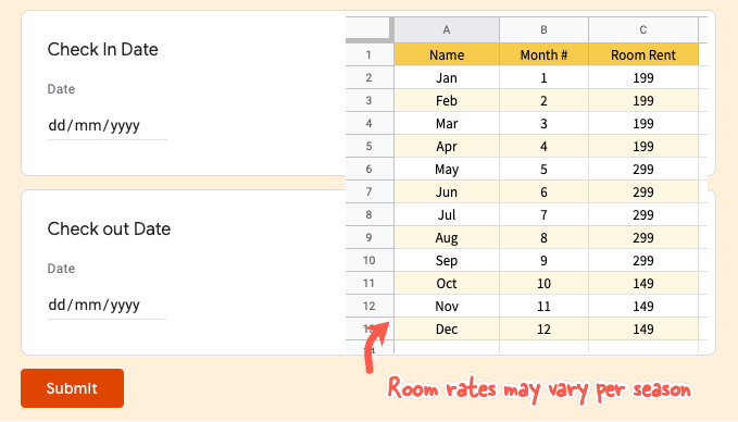
• For hotel reservations forms, a formula can automatically calculate the room rent based on the check-in and check-out date filled by the customer in the Google Form.
• For quizzes, a teacher can automatically calculate the final score of the student by matching the values entered in the form with the actual answers and assigning scores.
• If a users has made multiple form submissions, a formula can help you determine the total number of entries made by a user as soon as they submit a form.

Google Sheets Formulas for Google Forms

In this step by step guide, you’ll learn how to add formulas to Google Sheets that are associated with Google Forms. The corresponding cell values in the response rows will be automatically calculated when a new response is submitted.

To get a better understanding of what we are trying to achieve, open this Google Form and submit a response. Next, open this Google Sheet and you’ll find your response in a new row. The columns F-K are autofilled using formulas.

All examples below will use the ArrayFormula function of Google Sheets though some of these example can also be written using the FILTER function.

Auto-Number Form Responses with a Unique ID

Open the Google Sheet that is storing form responses, go to first empty column and copy-paste the following formula in the row #1 of the empty column.

=ArrayFormula(
  IFS(
    ROW(A:A)=1, "Invoice ID",
    LEN(A:A)=0, IFERROR(1/0),
    LEN(A:A)>0, LEFT(CONCAT(REPT("0",5), ROW(A:A) -1),6)
  )
)

The ROW() function returns the row number of the current response row. It returns 1 for the first row in the Invoice Column and thus we set the column title in the first row. For subsequent rows, if the first column of the row (usually Timestamp) is not empty, the invoice ID is auto generated.

The IDs will be like 00001, 00002 and so on. You only need to place the formula is first row of the column and it auto-populates all the other rows in the column.

The IFERROR function returns the first argument if it is not an error value, otherwise returns the second argument if present, or a blank if the second argument is absent. So in this case 1/0 is an error and thus it always returns a blank value.

Date Calculation Formula for Google Forms

Your Google Form has two date fields – the check-in date and the check-out date. The hotel rates may vary every season so you have a separate table in the Google Sheet that maintains the room rent per month.

The Column C in the Google Sheet holds the responses for the check-in date while the D column is storing the check-out dates.

=ArrayFormula(
    IF(ROW(A:A) = 1,
      "Room Rent",
      IF(NOT(ISBLANK(A:A)),
       (D:D - C:C) *
       VLOOKUP(MONTH(D:D), 'Room Rates'!$B$2:$C$13,2, TRUE),
       ""
      )
   )
)

The formulas uses VLOOKUP to get the room rates for the travel date specified in the form response and then calculates the room rent by multiplying the room rent with duration of stay.

The same formula can also be written with IFS instead of VLOOKUP

=ArrayFormula(
    IF(ROW(A:A) = 1,
        "Room Rent",
        IFS(ISBLANK(C:C), "",
           MONTH(C:C) < 2, 299,
           MONTH(C:C) < 5, 499,
           MONTH(C:C) < 9, 699,
           TRUE, 199
        )
    )
)

Calculate Tax Amount Based on Invoice Value

In this approach, we’ll use the FILTER function and that could lead to a less complicated formula than using using IF function. The downside is that you have to write the column title in row #1 and paste the formulas in row #2 (so one form response should exist for the formula to work).

=ArrayFormula(FILTER(E2:E, E2:E<>"")*1.35)

Here we apply 35% tax to the invoice value and this formula should be added in the row #2 of the column titled “Tax Amount” as shown in the screenshot.

Assign Quiz Scores in Google Forms

Which city is known as the big apple? This is a short-answer question in Google Forms so students can give responses like New York, New York City, NYC and they’ll still be correct. The teacher has to assign 10 points to the correct answer.

=ArrayFormula(
    IF(ROW(A:A) = 1,
      "Quiz Score",
      IFS(
        ISBLANK(A:A), "",
        REGEXMATCH(LOWER({B:B}), "news?york"), 10,
        {B:B} = "NYC", 10,
        TRUE, 0
      )
    )
)

In this formula, we are making use of the IFS function that like an IF THEN statement in programming. We are using REGEXMATCH to match values like New York, New York, newyork in one go using regular expressions.

The IFS function returns an NA if none of the conditions are true so we add a TRUE check at the end that will always be evaluated to true if none of the previous conditions matched and returns 0.

If you have form field that asks the user to entire their full name, you can use Google Sheets function to extract the first name from the full name and use that field to send personalised emails.

=ArrayFormula(
  IFS(
    ROW(A:A)=1, "First Name",
    LEN(A:A)=0, IFERROR(1/0),
    LEN(A:A)>0, PROPER(REGEXEXTRACT(B:B, "^[^s+]+"))
  )
)

We’ve used RegexExtract method here to fetch the string before the first space in the name field. The PROPER function will capitalise the first letter of the name incase the user entered their name in lower case.

Find Duplicate Google Form Submissions

If your Google Form is collection email addresses, you can use that field to quickly detect responses that have been submitted by the same user multiple times.

=ArrayFormula(
  IFS(
    ROW(A:A)=1, "Is Duplicate Entry?",
    LEN(A:A)=0, IFERROR(1/0),
    LEN(A:A)>0, IF(COUNTIF(B:B, B:B) > 1, "YES", "")
  )
)

Assuming that the Column B is storing the email addresses of the form respondents, we can use the COUNTIF function to quickly mark duplicate entries in our responses spreadsheet. You can also use conditional formatting in Sheets to highlight rows that are possible duplicate entries.

Email Form Responses with AutoFill Values

You can use Document Studio to automatically send an email to the form respondents. The email is sent after the formular values are auto-filled by the Google Sheet. The original form response and the calculated values can also be included in the generated PDF document.